Rebuilt graphs

The figures in the chapters are the ones pasted into the manuscript in 2005 — mostly 480×480 bitmaps, which is why they look soft.

These are the same graphs drawn again from the data itself. The MATLAB .fig files kept the coordinates, not just a picture of them, so the curves could simply be replotted — as vector, which stays sharp at any zoom. 36 of the 39 files still held usable data.

Each one shows the Python that draws it, which was the original idea for this book: put the plotting language next to the mathematics.

A cylinder

The Python that draws it

import json
import numpy as np
import matplotlib.pyplot as plt

# Surface recovered from the 2005 MATLAB figure "cilindru".
# The mesh is 2x41, so the data ships alongside
# rather than being printed here.
data = json.load(open("cilindru.json"))["series"][0]
X = np.array(data["x"]).reshape(data["x_shape"])
Y = np.array(data["y"]).reshape(data["y_shape"])
Z = np.array(data["z"], dtype=float)

fig = plt.figure(figsize=(6.4, 4.8))
ax = fig.add_subplot(111, projection="3d")
ax.plot_surface(X, Y, Z, cmap="viridis", linewidth=0)
ax.set_box_aspect((1, 1, 0.7))
fig.savefig("cilindru.svg")    # SVG: sharp at any zoom

It reads its data from cilindru.json — save that next to the script.

From the 2005 figure cilindru.

Horizontal compression

The same curve compressed along the x-axis.

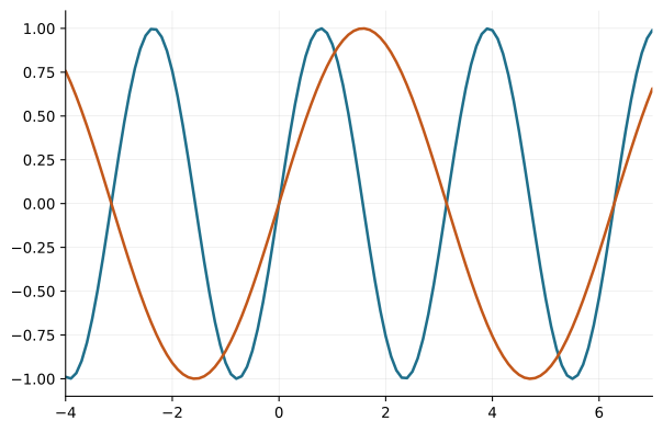
The Python that draws it

import numpy as np
import matplotlib.pyplot as plt

# 2 curve(s) recovered from the 2005 MATLAB figure "comprimare"
import json
series = json.load(open("comprimare.json"))["series"]

fig, ax = plt.subplots(figsize=(6.4, 4.2))
for s in series:
    ax.plot(s["x"], s["y"], lw=1.9)
ax.grid(True, lw=0.4, alpha=0.35)
ax.set_xlim(-4, 7)
ax.set_ylim(-1.1, 1.1)
ax.set_xlabel("x"); ax.set_ylabel("y")
fig.savefig("comprimare.svg")    # SVG: sharp at any zoom

It reads its data from comprimare.json — save that next to the script.

From the 2005 figure comprimare.

A cone as a solid of revolution

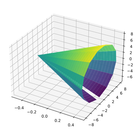
The Python that draws it

import json
import numpy as np
import matplotlib.pyplot as plt

# Surface recovered from the 2005 MATLAB figure "con(rot)".
# The mesh is 81x41, so the data ships alongside
# rather than being printed here.
data = json.load(open("con-rot-.json"))["series"][0]
X = np.array(data["x"]).reshape(data["x_shape"])
Y = np.array(data["y"]).reshape(data["y_shape"])
Z = np.array(data["z"], dtype=float)

fig = plt.figure(figsize=(6.4, 4.8))
ax = fig.add_subplot(111, projection="3d")
ax.plot_surface(X, Y, Z, cmap="viridis", linewidth=0)
ax.set_box_aspect((1, 1, 0.7))
fig.savefig("con-rot-.svg")    # SVG: sharp at any zoom

It reads its data from con-rot-.json — save that next to the script.

From the 2005 figure con-rot-.

Newton's law of cooling

A body cooling towards the temperature of its surroundings.

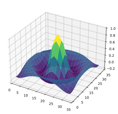
The Python that draws it

import json
import numpy as np
import matplotlib.pyplot as plt

# Surface recovered from the 2005 MATLAB figure "cool".
# The mesh is 33x33, so the data ships alongside
# rather than being printed here.
data = json.load(open("cool.json"))["series"][0]
X = np.array(data["x"]).reshape(data["x_shape"])
Y = np.array(data["y"]).reshape(data["y_shape"])
Z = np.array(data["z"], dtype=float)

fig = plt.figure(figsize=(6.4, 4.8))
ax = fig.add_subplot(111, projection="3d")
ax.plot_surface(X, Y, Z, cmap="viridis", linewidth=0)
ax.set_box_aspect((1, 1, 0.7))
fig.savefig("cool.svg")    # SVG: sharp at any zoom

It reads its data from cool.json — save that next to the script.

From the 2005 figure cool.

The damped cotangent

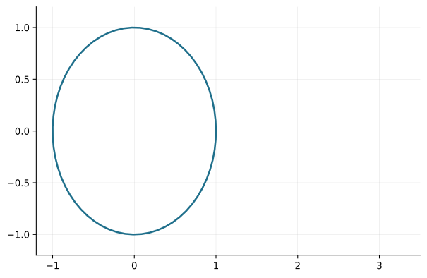
The Python that draws it

import numpy as np
import matplotlib.pyplot as plt

# 1 curve(s) recovered from the 2005 MATLAB figure "cotan1"
import json
series = json.load(open("cotan1.json"))["series"]

fig, ax = plt.subplots(figsize=(6.4, 4.2))
for s in series:
    ax.plot(s["x"], s["y"], lw=1.9)
ax.grid(True, lw=0.4, alpha=0.35)
ax.set_xlim(-1.2, 3.5)
ax.set_ylim(-1.2, 1.2)
ax.set_xlabel("x"); ax.set_ylabel("y")
fig.savefig("cotan1.svg")    # SVG: sharp at any zoom

It reads its data from cotan1.json — save that next to the script.

From the 2005 figure cotan1.

Solution of a differential equation

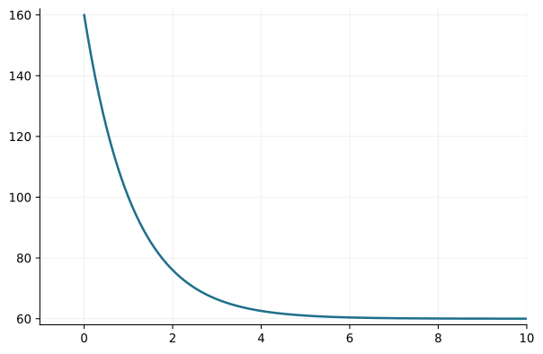
The Python that draws it

import numpy as np
import matplotlib.pyplot as plt

# 1 curve(s) recovered from the 2005 MATLAB figure "ecdif"
import json
series = json.load(open("ecdif.json"))["series"]

fig, ax = plt.subplots(figsize=(6.4, 4.2))
for s in series:
    ax.plot(s["x"], s["y"], lw=1.9)
ax.grid(True, lw=0.4, alpha=0.35)
ax.set_xlim(-1, 10)
ax.set_ylim(58, 162)
ax.set_xlabel("x"); ax.set_ylabel("y")
fig.savefig("ecdif.svg")    # SVG: sharp at any zoom

It reads its data from ecdif.json — save that next to the script.

From the 2005 figure ecdif.

Area between two curves

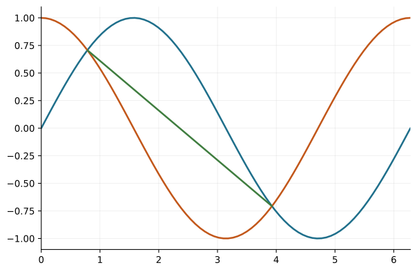
The Python that draws it

import numpy as np
import matplotlib.pyplot as plt

# 3 curve(s) recovered from the 2005 MATLAB figure "intergraf"
import json
series = json.load(open("intergraf.json"))["series"]

fig, ax = plt.subplots(figsize=(6.4, 4.2))
for s in series:
    ax.plot(s["x"], s["y"], lw=1.9)
ax.grid(True, lw=0.4, alpha=0.35)
ax.set_xlim(0, 6.28318)
ax.set_ylim(-1.1, 1.1)
ax.set_xlabel("x"); ax.set_ylabel("y")
fig.savefig("intergraf.svg")    # SVG: sharp at any zoom

It reads its data from intergraf.json — save that next to the script.

From the 2005 figure intergraf.

Area between two curves

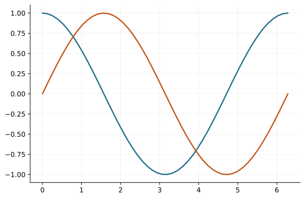
The Python that draws it

import numpy as np
import matplotlib.pyplot as plt

# 2 curve(s) recovered from the 2005 MATLAB figure "intergraf1"

x1 = np.array([
    0, 0.128228, 0.256457, 0.384685, 0.512913, 0.641141, 0.76937, 0.897598,
    1.02583, 1.15405, 1.28228, 1.41051, 1.53874, 1.66697, 1.7952, 1.92342,
    2.05165, 2.17988, 2.30811, 2.43634, 2.56456, 2.69279, 2.82102, 2.94925,
    3.07748, 3.20571, 3.33393, 3.46216, 3.59039, 3.71862, 3.84685, 3.97508,
    4.1033, 4.23153, 4.35976, 4.48799, 4.61622, 4.74445, 4.87267, 5.0009,
    5.12913, 5.25736, 5.38559, 5.51382, 5.64204, 5.77027, 5.8985, 6.02673,
    6.15496, 6.28318
])
y1 = np.array([
    1, 0.99179, 0.967295, 0.926917, 0.871319, 0.801414, 0.718349, 0.62349,
    0.518393, 0.404783, 0.284528, 0.1596, 0.032052, -0.096023, -0.222521,
    -0.345365, -0.462538, -0.572117, -0.672301, -0.761446, -0.838088,
    -0.900969, -0.949056, -0.981559, -0.997945, -0.997945, -0.981559,
    -0.949056, -0.900969, -0.838088, -0.761446, -0.672301, -0.572117,
    -0.462538, -0.345365, -0.222521, -0.096023, 0.032052, 0.1596, 0.284528,
    0.404783, 0.518393, 0.62349, 0.718349, 0.801414, 0.871319, 0.926917,
    0.967295, 0.99179, 1
])

x2 = np.array([
    0, 0.128228, 0.256457, 0.384685, 0.512913, 0.641141, 0.76937, 0.897598,
    1.02583, 1.15405, 1.28228, 1.41051, 1.53874, 1.66697, 1.7952, 1.92342,
    2.05165, 2.17988, 2.30811, 2.43634, 2.56456, 2.69279, 2.82102, 2.94925,
    3.07748, 3.20571, 3.33393, 3.46216, 3.59039, 3.71862, 3.84685, 3.97508,
    4.1033, 4.23153, 4.35976, 4.48799, 4.61622, 4.74445, 4.87267, 5.0009,
    5.12913, 5.25736, 5.38559, 5.51382, 5.64204, 5.77027, 5.8985, 6.02673,
    6.15496, 6.28318
])
y2 = np.array([
    0, 0.127877, 0.253655, 0.375267, 0.490718, 0.598111, 0.695683, 0.781831,
    0.855143, 0.914413, 0.958668, 0.987182, 0.999486, 0.995379, 0.974928,
    0.938468, 0.886599, 0.820172, 0.740278, 0.648228, 0.545535, 0.433884,
    0.315108, 0.191159, 0.06407, -0.06407, -0.191159, -0.315108, -0.433884,
    -0.545535, -0.648228, -0.740278, -0.820172, -0.886599, -0.938468,
    -0.974928, -0.995379, -0.999486, -0.987182, -0.958668, -0.914413,
    -0.855143, -0.781831, -0.695683, -0.598111, -0.490718, -0.375267,
    -0.253655, -0.127877, -0
])

fig, ax = plt.subplots(figsize=(6.4, 4.2))
ax.plot(x1, y1, lw=1.9)
ax.plot(x2, y2, lw=1.9)
ax.grid(True, lw=0.4, alpha=0.35)
ax.set_xlabel("x"); ax.set_ylabel("y")
fig.savefig("intergraf1.svg")    # SVG: sharp at any zoom

From the 2005 figure intergraf1.

Area between two curves

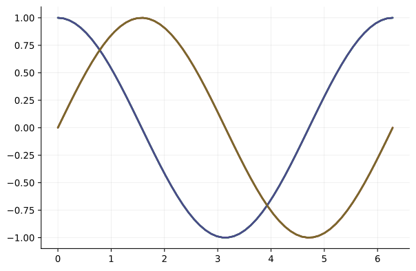
The Python that draws it

import numpy as np
import matplotlib.pyplot as plt

# 6 curve(s) recovered from the 2005 MATLAB figure "intergraf2"

x1 = np.array([
    0, 0.106495, 0.212989, 0.319484, 0.425979, 0.532473, 0.638968, 0.745463,
    0.851957, 0.958452, 1.06495, 1.17144, 1.27794, 1.38443, 1.49093, 1.59742,
    1.70392, 1.81041, 1.9169, 2.0234, 2.12989, 2.23639, 2.34288, 2.44938,
    2.55587, 2.66237, 2.76886, 2.87536, 2.98185, 3.08834, 3.19484, 3.30133,
    3.40783, 3.51432, 3.62082, 3.72731, 3.83381, 3.9403, 4.0468, 4.15329,
    4.25979, 4.36628, 4.47278, 4.57927, 4.68576, 4.79226, 4.89876, 5.00525,
    5.11174, 5.21824, 5.32473, 5.43123, 5.53772, 5.64422, 5.75071, 5.85721,
    5.9637, 6.0702, 6.17669, 6.28318
])
y1 = np.array([
    1, 0.994335, 0.977403, 0.949398, 0.910635, 0.861554, 0.802712, 0.734774,
    0.658511, 0.574787, 0.484551, 0.388824, 0.288692, 0.185289, 0.079786,
    -0.026621, -0.132726, -0.237327, -0.339239, -0.437307, -0.530421,
    -0.617525, -0.697632, -0.769834, -0.833314, -0.887352, -0.931336,
    -0.964768, -0.987268, -0.998583, -0.998583, -0.987268, -0.964768,
    -0.931336, -0.887352, -0.833314, -0.769834, -0.697632, -0.617525,
    -0.530421, -0.437307, -0.339239, -0.237327, -0.132726, -0.026621,
    0.079786, 0.185289, 0.288692, 0.388824, 0.484551, 0.574787, 0.658511,
    0.734774, 0.802712, 0.861554, 0.910635, 0.949398, 0.977403, 0.994335, 1
])

x2 = np.array([
    0, 0.106495, 0.212989, 0.319484, 0.425979, 0.532473, 0.638968, 0.745463,
    0.851957, 0.958452, 1.06495, 1.17144, 1.27794, 1.38443, 1.49093, 1.59742,
    1.70392, 1.81041, 1.9169, 2.0234, 2.12989, 2.23639, 2.34288, 2.44938,
    2.55587, 2.66237, 2.76886, 2.87536, 2.98185, 3.08834, 3.19484, 3.30133,
    3.40783, 3.51432, 3.62082, 3.72731, 3.83381, 3.9403, 4.0468, 4.15329,
    4.25979, 4.36628, 4.47278, 4.57927, 4.68576, 4.79226, 4.89876, 5.00525,
    5.11174, 5.21824, 5.32473, 5.43123, 5.53772, 5.64422, 5.75071, 5.85721,
    5.9637, 6.0702, 6.17669, 6.28318
])
y2 = np.array([
    0, 0.106293, 0.211383, 0.314077, 0.413212, 0.507666, 0.596367, 0.678312,
    0.752571, 0.818303, 0.874763, 0.921312, 0.957422, 0.982684, 0.996812,
    0.999646, 0.991153, 0.97143, 0.9407, 0.899312, 0.847734, 0.786552,
    0.716457, 0.638244, 0.5528, 0.461093, 0.364161, 0.263103, 0.159063,
    0.053222, -0.053222, -0.159063, -0.263103, -0.364161, -0.461093, -0.5528,
    -0.638244, -0.716457, -0.786552, -0.847734, -0.899312, -0.9407, -0.97143,
    -0.991153, -0.999646, -0.996812, -0.982684, -0.957422, -0.921312,
    -0.874763, -0.818303, -0.752571, -0.678312, -0.596367, -0.507666,
    -0.413212, -0.314077, -0.211383, -0.106293, -0
])

x3 = np.array([
    0, 0.106495, 0.212989, 0.319484, 0.425979, 0.532473, 0.638968, 0.745463,
    0.851957, 0.958452, 1.06495, 1.17144, 1.27794, 1.38443, 1.49093, 1.59742,
    1.70392, 1.81041, 1.9169, 2.0234, 2.12989, 2.23639, 2.34288, 2.44938,
    2.55587, 2.66237, 2.76886, 2.87536, 2.98185, 3.08834, 3.19484, 3.30133,
    3.40783, 3.51432, 3.62082, 3.72731, 3.83381, 3.9403, 4.0468, 4.15329,
    4.25979, 4.36628, 4.47278, 4.57927, 4.68576, 4.79226, 4.89876, 5.00525,
    5.11174, 5.21824, 5.32473, 5.43123, 5.53772, 5.64422, 5.75071, 5.85721,
    5.9637, 6.0702, 6.17669, 6.28318
])
y3 = np.array([
    1, 0.994335, 0.977403, 0.949398, 0.910635, 0.861554, 0.802712, 0.734774,
    0.658511, 0.574787, 0.484551, 0.388824, 0.288692, 0.185289, 0.079786,
    -0.026621, -0.132726, -0.237327, -0.339239, -0.437307, -0.530421,
    -0.617525, -0.697632, -0.769834, -0.833314, -0.887352, -0.931336,
    -0.964768, -0.987268, -0.998583, -0.998583, -0.987268, -0.964768,
    -0.931336, -0.887352, -0.833314, -0.769834, -0.697632, -0.617525,
    -0.530421, -0.437307, -0.339239, -0.237327, -0.132726, -0.026621,
    0.079786, 0.185289, 0.288692, 0.388824, 0.484551, 0.574787, 0.658511,
    0.734774, 0.802712, 0.861554, 0.910635, 0.949398, 0.977403, 0.994335, 1
])

x4 = np.array([
    0, 0.106495, 0.212989, 0.319484, 0.425979, 0.532473, 0.638968, 0.745463,
    0.851957, 0.958452, 1.06495, 1.17144, 1.27794, 1.38443, 1.49093, 1.59742,
    1.70392, 1.81041, 1.9169, 2.0234, 2.12989, 2.23639, 2.34288, 2.44938,
    2.55587, 2.66237, 2.76886, 2.87536, 2.98185, 3.08834, 3.19484, 3.30133,
    3.40783, 3.51432, 3.62082, 3.72731, 3.83381, 3.9403, 4.0468, 4.15329,
    4.25979, 4.36628, 4.47278, 4.57927, 4.68576, 4.79226, 4.89876, 5.00525,
    5.11174, 5.21824, 5.32473, 5.43123, 5.53772, 5.64422, 5.75071, 5.85721,
    5.9637, 6.0702, 6.17669, 6.28318
])
y4 = np.array([
    0, 0.106293, 0.211383, 0.314077, 0.413212, 0.507666, 0.596367, 0.678312,
    0.752571, 0.818303, 0.874763, 0.921312, 0.957422, 0.982684, 0.996812,
    0.999646, 0.991153, 0.97143, 0.9407, 0.899312, 0.847734, 0.786552,
    0.716457, 0.638244, 0.5528, 0.461093, 0.364161, 0.263103, 0.159063,
    0.053222, -0.053222, -0.159063, -0.263103, -0.364161, -0.461093, -0.5528,
    -0.638244, -0.716457, -0.786552, -0.847734, -0.899312, -0.9407, -0.97143,
    -0.991153, -0.999646, -0.996812, -0.982684, -0.957422, -0.921312,
    -0.874763, -0.818303, -0.752571, -0.678312, -0.596367, -0.507666,
    -0.413212, -0.314077, -0.211383, -0.106293, -0
])

x5 = np.array([
    0, 0.106495, 0.212989, 0.319484, 0.425979, 0.532473, 0.638968, 0.745463,
    0.851957, 0.958452, 1.06495, 1.17144, 1.27794, 1.38443, 1.49093, 1.59742,
    1.70392, 1.81041, 1.9169, 2.0234, 2.12989, 2.23639, 2.34288, 2.44938,
    2.55587, 2.66237, 2.76886, 2.87536, 2.98185, 3.08834, 3.19484, 3.30133,
    3.40783, 3.51432, 3.62082, 3.72731, 3.83381, 3.9403, 4.0468, 4.15329,
    4.25979, 4.36628, 4.47278, 4.57927, 4.68576, 4.79226, 4.89876, 5.00525,
    5.11174, 5.21824, 5.32473, 5.43123, 5.53772, 5.64422, 5.75071, 5.85721,
    5.9637, 6.0702, 6.17669, 6.28318
])
y5 = np.array([
    1, 0.994335, 0.977403, 0.949398, 0.910635, 0.861554, 0.802712, 0.734774,
    0.658511, 0.574787, 0.484551, 0.388824, 0.288692, 0.185289, 0.079786,
    -0.026621, -0.132726, -0.237327, -0.339239, -0.437307, -0.530421,
    -0.617525, -0.697632, -0.769834, -0.833314, -0.887352, -0.931336,
    -0.964768, -0.987268, -0.998583, -0.998583, -0.987268, -0.964768,
    -0.931336, -0.887352, -0.833314, -0.769834, -0.697632, -0.617525,
    -0.530421, -0.437307, -0.339239, -0.237327, -0.132726, -0.026621,
    0.079786, 0.185289, 0.288692, 0.388824, 0.484551, 0.574787, 0.658511,
    0.734774, 0.802712, 0.861554, 0.910635, 0.949398, 0.977403, 0.994335, 1
])

x6 = np.array([
    0, 0.106495, 0.212989, 0.319484, 0.425979, 0.532473, 0.638968, 0.745463,
    0.851957, 0.958452, 1.06495, 1.17144, 1.27794, 1.38443, 1.49093, 1.59742,
    1.70392, 1.81041, 1.9169, 2.0234, 2.12989, 2.23639, 2.34288, 2.44938,
    2.55587, 2.66237, 2.76886, 2.87536, 2.98185, 3.08834, 3.19484, 3.30133,
    3.40783, 3.51432, 3.62082, 3.72731, 3.83381, 3.9403, 4.0468, 4.15329,
    4.25979, 4.36628, 4.47278, 4.57927, 4.68576, 4.79226, 4.89876, 5.00525,
    5.11174, 5.21824, 5.32473, 5.43123, 5.53772, 5.64422, 5.75071, 5.85721,
    5.9637, 6.0702, 6.17669, 6.28318
])
y6 = np.array([
    0, 0.106293, 0.211383, 0.314077, 0.413212, 0.507666, 0.596367, 0.678312,
    0.752571, 0.818303, 0.874763, 0.921312, 0.957422, 0.982684, 0.996812,
    0.999646, 0.991153, 0.97143, 0.9407, 0.899312, 0.847734, 0.786552,
    0.716457, 0.638244, 0.5528, 0.461093, 0.364161, 0.263103, 0.159063,
    0.053222, -0.053222, -0.159063, -0.263103, -0.364161, -0.461093, -0.5528,
    -0.638244, -0.716457, -0.786552, -0.847734, -0.899312, -0.9407, -0.97143,
    -0.991153, -0.999646, -0.996812, -0.982684, -0.957422, -0.921312,
    -0.874763, -0.818303, -0.752571, -0.678312, -0.596367, -0.507666,
    -0.413212, -0.314077, -0.211383, -0.106293, -0
])

fig, ax = plt.subplots(figsize=(6.4, 4.2))
ax.plot(x1, y1, lw=1.9)
ax.plot(x2, y2, lw=1.9)
ax.plot(x3, y3, lw=1.9)
ax.plot(x4, y4, lw=1.9)
ax.plot(x5, y5, lw=1.9)
ax.plot(x6, y6, lw=1.9)
ax.grid(True, lw=0.4, alpha=0.35)
ax.set_xlabel("x"); ax.set_ylabel("y")
fig.savefig("intergraf2.svg")    # SVG: sharp at any zoom

From the 2005 figure intergraf2.

Area between two curves

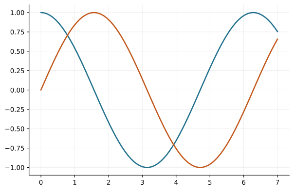
The Python that draws it

import numpy as np
import matplotlib.pyplot as plt

# 2 curve(s) recovered from the 2005 MATLAB figure "intergraf3"
import json
series = json.load(open("intergraf3.json"))["series"]

fig, ax = plt.subplots(figsize=(6.4, 4.2))
for s in series:
    ax.plot(s["x"], s["y"], lw=1.9)
ax.grid(True, lw=0.4, alpha=0.35)
ax.set_xlabel("x"); ax.set_ylabel("y")
fig.savefig("intergraf3.svg")    # SVG: sharp at any zoom

It reads its data from intergraf3.json — save that next to the script.

From the 2005 figure intergraf3.

Area under y = √x

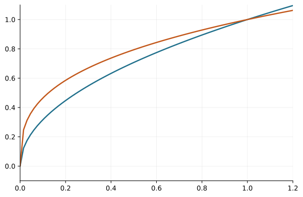
The Python that draws it

import numpy as np
import matplotlib.pyplot as plt

# 2 curve(s) recovered from the 2005 MATLAB figure "intergrfsqrt"
import json
series = json.load(open("intergrfsqrt.json"))["series"]

fig, ax = plt.subplots(figsize=(6.4, 4.2))
for s in series:
    ax.plot(s["x"], s["y"], lw=1.9)
ax.grid(True, lw=0.4, alpha=0.35)
ax.set_xlim(0, 1.2)
ax.set_ylim(-0.1, 1.1)
ax.set_xlabel("x"); ax.set_ylabel("y")
fig.savefig("intergrfsqrt.svg")    # SVG: sharp at any zoom

It reads its data from intergrfsqrt.json — save that next to the script.

From the 2005 figure intergrfsqrt.

Area under y = x³

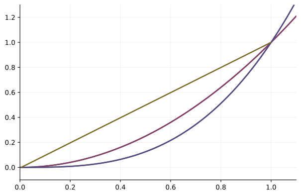
The Python that draws it

import numpy as np
import matplotlib.pyplot as plt

# 6 curve(s) recovered from the 2005 MATLAB figure "intergrfx3"
import json
series = json.load(open("intergrfx3.json"))["series"]

fig, ax = plt.subplots(figsize=(6.4, 4.2))
for s in series:
    ax.plot(s["x"], s["y"], lw=1.9)
ax.grid(True, lw=0.4, alpha=0.35)
ax.set_xlim(0, 1.1)
ax.set_ylim(-0.1, 1.3)
ax.set_xlabel("x"); ax.set_ylabel("y")
fig.savefig("intergrfx3.svg")    # SVG: sharp at any zoom

It reads its data from intergrfx3.json — save that next to the script.

From the 2005 figure intergrfx3.

Area between y = x² and y = x

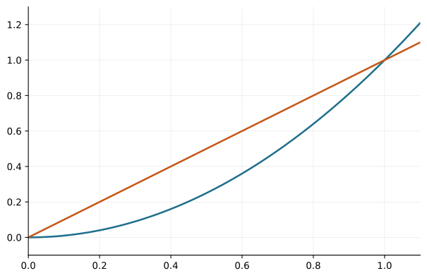
The Python that draws it

import numpy as np
import matplotlib.pyplot as plt

# 2 curve(s) recovered from the 2005 MATLAB figure "interx2x"
import json
series = json.load(open("interx2x.json"))["series"]

fig, ax = plt.subplots(figsize=(6.4, 4.2))
for s in series:
    ax.plot(s["x"], s["y"], lw=1.9)
ax.grid(True, lw=0.4, alpha=0.35)
ax.set_xlim(0, 1.1)
ax.set_ylim(-0.1, 1.3)
ax.set_xlabel("x"); ax.set_ylabel("y")
fig.savefig("interx2x.svg")    # SVG: sharp at any zoom

It reads its data from interx2x.json — save that next to the script.

From the 2005 figure interx2x.

A function and its inverse

y = x² and y = √x are mirror images in the line y = x.

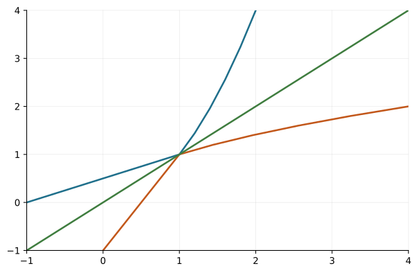
The Python that draws it

import numpy as np
import matplotlib.pyplot as plt

# 3 curve(s) recovered from the 2005 MATLAB figure "inverse"

x1 = np.array([
    -1, -0.8, -0.6, -0.4, -0.2, 0, 0.2, 0.4, 0.6, 0.8, 1, 1.2, 1.4, 1.6, 1.8,
    2, 2.2, 2.4, 2.6, 2.8, 3, 3.2, 3.4, 3.6, 3.8, 4
])
y1 = np.array([
    0, 0.1, 0.2, 0.3, 0.4, 0.5, 0.6, 0.7, 0.8, 0.9, 1, 1.44, 1.96, 2.56,
    3.24, 4, 4.84, 5.76, 6.76, 7.84, 9, 10.24, 11.56, 12.96, 14.44, 16
])

x2 = np.array([
    0, 0.1, 0.2, 0.3, 0.4, 0.5, 0.6, 0.7, 0.8, 0.9, 1, 1.44, 1.96, 2.56,
    3.24, 4, 4.84, 5.76, 6.76, 7.84, 9, 10.24, 11.56, 12.96, 14.44, 16
])
y2 = np.array([
    -1, -0.8, -0.6, -0.4, -0.2, 0, 0.2, 0.4, 0.6, 0.8, 1, 1.2, 1.4, 1.6, 1.8,
    2, 2.2, 2.4, 2.6, 2.8, 3, 3.2, 3.4, 3.6, 3.8, 4
])

x3 = np.array([
    -1, -0.8, -0.6, -0.4, -0.2, 0, 0.2, 0.4, 0.6, 0.8, 1, 1.2, 1.4, 1.6, 1.8,
    2, 2.2, 2.4, 2.6, 2.8, 3, 3.2, 3.4, 3.6, 3.8, 4
])
y3 = np.array([
    -1, -0.8, -0.6, -0.4, -0.2, 0, 0.2, 0.4, 0.6, 0.8, 1, 1.2, 1.4, 1.6, 1.8,
    2, 2.2, 2.4, 2.6, 2.8, 3, 3.2, 3.4, 3.6, 3.8, 4
])

fig, ax = plt.subplots(figsize=(6.4, 4.2))
ax.plot(x1, y1, lw=1.9)
ax.plot(x2, y2, lw=1.9)
ax.plot(x3, y3, lw=1.9)
ax.grid(True, lw=0.4, alpha=0.35)
ax.set_xlim(-1, 4)
ax.set_ylim(-1, 4)
ax.set_xlabel("x"); ax.set_ylabel("y")
fig.savefig("inverse.svg")    # SVG: sharp at any zoom

From the 2005 figure inverse.

A logarithm curve

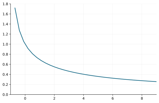
The Python that draws it

import numpy as np
import matplotlib.pyplot as plt

# 1 curve(s) recovered from the 2005 MATLAB figure "lnc2"

x1 = np.array([
    -1, -0.7, -0.4, -0.1, 0.2, 0.5, 0.8, 1.1, 1.4, 1.7, 2, 2.3, 2.6, 2.9,
    3.2, 3.5, 3.8, 4.1, 4.4, 4.7, 5, 5.3, 5.6, 5.9, 6.2, 6.5, 6.8, 7.1, 7.4,
    7.7, 8, 8.3, 8.6, 8.9, 9.2, 9.5, 9.8
])
y1 = np.array([
    np.nan, 1.71996, 1.27706, 1.0536, 0.911608, 0.81093, 0.734733, 0.674488,
    0.625335, 0.584266, 0.549306, 0.519097, 0.492667, 0.469302, 0.448464,
    0.429736, 0.412794, 0.397376, 0.383272, 0.370312, 0.358352, 0.347274,
    0.336977, 0.327377, 0.3184, 0.309985, 0.302077, 0.294629, 0.287599,
    0.280951, 0.274653, 0.268676, 0.262996, 0.257588, 0.252433, 0.247513,
    0.242811
])

fig, ax = plt.subplots(figsize=(6.4, 4.2))
ax.plot(x1, y1, lw=1.9)
ax.grid(True, lw=0.4, alpha=0.35)
ax.set_xlim(-1, 9)
ax.set_ylim(0, 1.8)
ax.set_xlabel("x"); ax.set_ylabel("y")
fig.savefig("lnc2.svg")    # SVG: sharp at any zoom

From the 2005 figure lnc2.

Minimum and maximum on a graph

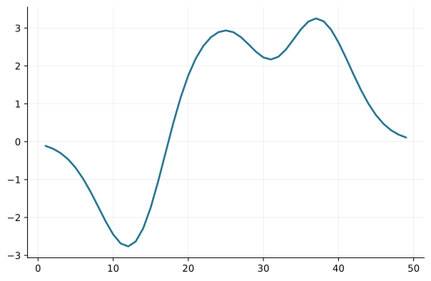
The Python that draws it

import numpy as np
import matplotlib.pyplot as plt

# 1 curve(s) recovered from the 2005 MATLAB figure "mixsimaxpegraf"

x1 = np.array([
    1, 2, 3, 4, 5, 6, 7, 8, 9, 10, 11, 12, 13, 14, 15, 16, 17, 18, 19, 20,
    21, 22, 23, 24, 25, 26, 27, 28, 29, 30, 31, 32, 33, 34, 35, 36, 37, 38,
    39, 40, 41, 42, 43, 44, 45, 46, 47, 48, 49
])
y1 = np.array([
    -0.109959, -0.185102, -0.299093, -0.463448, -0.68786, -0.976604,
    -1.32418, -1.71125, -2.10235, -2.4472, -2.68667, -2.76333, -2.63487,
    -2.28639, -1.73765, -1.04148, -0.272917, 0.488316, 1.17599, 1.74984,
    2.19775, 2.52795, 2.75562, 2.89129, 2.93693, 2.89151, 2.76237, 2.57535,
    2.37682, 2.22462, 2.17083, 2.24328, 2.43379, 2.69828, 2.96888, 3.17321,
    3.25397, 3.18224, 2.96139, 2.62183, 2.20994, 1.77549, 1.36136, 0.99746,
    0.699199, 0.469423, 0.302145, 0.186613, 0.110684
])

fig, ax = plt.subplots(figsize=(6.4, 4.2))
ax.plot(x1, y1, lw=1.9)
ax.grid(True, lw=0.4, alpha=0.35)
ax.set_xlabel("x"); ax.set_ylabel("y")
fig.savefig("mixsimaxpegraf.svg")    # SVG: sharp at any zoom

From the 2005 figure mixsimaxpegraf.

Several curves together

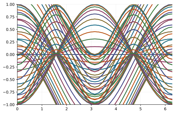
The Python that draws it

import numpy as np
import matplotlib.pyplot as plt

# 6 curve(s) recovered from the 2005 MATLAB figure "multipleplots"

x1 = np.array([
    0, 0.156434, 0.309017, 0.45399, 0.587785, 0.707107, 0.809017, 0.891007,
    0.951057, 0.987688, 1, 0.987688, 0.951057, 0.891007, 0.809017, 0.707107,
    0.587785, 0.45399, 0.309017, 0.156434, 0, -0.156434, -0.309017, -0.45399,
    -0.587785, -0.707107, -0.809017, -0.891007, -0.951057, -0.987688, -1,
    -0.987688, -0.951057, -0.891007, -0.809017, -0.707107, -0.587785,
    -0.45399, -0.309017, -0.156434, -0
])
y1 = np.array([
    1, 0.987688, 0.951057, 0.891007, 0.809017, 0.707107, 0.587785, 0.45399,
    0.309017, 0.156434, 0, -0.156434, -0.309017, -0.45399, -0.587785,
    -0.707107, -0.809017, -0.891007, -0.951057, -0.987688, -1, -0.987688,
    -0.951057, -0.891007, -0.809017, -0.707107, -0.587785, -0.45399,
    -0.309017, -0.156434, -0, 0.156434, 0.309017, 0.45399, 0.587785,
    0.707107, 0.809017, 0.891007, 0.951057, 0.987688, 1
])

x2 = np.array([
    0, 0.15708, 0.314159, 0.471239, 0.628319, 0.785398, 0.942478, 1.09956,
    1.25664, 1.41372, 1.5708, 1.72788, 1.88496, 2.04203, 2.19911, 2.35619,
    2.51327, 2.67035, 2.82743, 2.98451, 3.14159, 3.29867, 3.45575, 3.61283,
    3.76991, 3.92699, 4.08407, 4.24115, 4.39823, 4.55531, 4.71239, 4.86947,
    5.02655, 5.18363, 5.34071, 5.49779, 5.65487, 5.81195, 5.96903, 6.12611,
    6.28318
])
y2 = np.array([
    1, 0.987688, 0.951057, 0.891007, 0.809017, 0.707107, 0.587785, 0.45399,
    0.309017, 0.156434, 0, -0.156434, -0.309017, -0.45399, -0.587785,
    -0.707107, -0.809017, -0.891007, -0.951057, -0.987688, -1, -0.987688,
    -0.951057, -0.891007, -0.809017, -0.707107, -0.587785, -0.45399,
    -0.309017, -0.156434, -0, 0.156434, 0.309017, 0.45399, 0.587785,
    0.707107, 0.809017, 0.891007, 0.951057, 0.987688, 1
])

x3 = np.array([
    0, 0.15708, 0.314159, 0.471239, 0.628319, 0.785398, 0.942478, 1.09956,
    1.25664, 1.41372, 1.5708, 1.72788, 1.88496, 2.04203, 2.19911, 2.35619,
    2.51327, 2.67035, 2.82743, 2.98451, 3.14159, 3.29867, 3.45575, 3.61283,
    3.76991, 3.92699, 4.08407, 4.24115, 4.39823, 4.55531, 4.71239, 4.86947,
    5.02655, 5.18363, 5.34071, 5.49779, 5.65487, 5.81195, 5.96903, 6.12611,
    6.28318
])
y3 = np.array([
    1.15643, 1.14412, 1.10749, 1.04744, 0.965451, 0.863541, 0.74422,
    0.610425, 0.465451, 0.312869, 0.156434, 0, -0.152583, -0.297556,
    -0.431351, -0.550672, -0.652583, -0.734572, -0.794622, -0.831254,
    -0.843566, -0.831254, -0.794622, -0.734572, -0.652583, -0.550672,
    -0.431351, -0.297556, -0.152583, -0, 0.156434, 0.312869, 0.465451,
    0.610425, 0.74422, 0.863541, 0.965451, 1.04744, 1.10749, 1.14412,
    1.15643
])

x4 = np.array([
    0, 0.15708, 0.314159, 0.471239, 0.628319, 0.785398, 0.942478, 1.09956,
    1.25664, 1.41372, 1.5708, 1.72788, 1.88496, 2.04203, 2.19911, 2.35619,
    2.51327, 2.67035, 2.82743, 2.98451, 3.14159, 3.29867, 3.45575, 3.61283,
    3.76991, 3.92699, 4.08407, 4.24115, 4.39823, 4.55531, 4.71239, 4.86947,
    5.02655, 5.18363, 5.34071, 5.49779, 5.65487, 5.81195, 5.96903, 6.12611,
    6.28318
])
y4 = np.array([
    1.30902, 1.2967, 1.26007, 1.20002, 1.11803, 1.01612, 0.896802, 0.763007,
    0.618034, 0.465451, 0.309017, 0.152583, 0, -0.144974, -0.278768,
    -0.39809, -0.5, -0.58199, -0.64204, -0.678671, -0.690983, -0.678671,
    -0.64204, -0.58199, -0.5, -0.39809, -0.278768, -0.144974, -0, 0.152583,
    0.309017, 0.465451, 0.618034, 0.763007, 0.896802, 1.01612, 1.11803,
    1.20002, 1.26007, 1.2967, 1.30902
])

x5 = np.array([
    0, 0.15708, 0.314159, 0.471239, 0.628319, 0.785398, 0.942478, 1.09956,
    1.25664, 1.41372, 1.5708, 1.72788, 1.88496, 2.04203, 2.19911, 2.35619,
    2.51327, 2.67035, 2.82743, 2.98451, 3.14159, 3.29867, 3.45575, 3.61283,
    3.76991, 3.92699, 4.08407, 4.24115, 4.39823, 4.55531, 4.71239, 4.86947,
    5.02655, 5.18363, 5.34071, 5.49779, 5.65487, 5.81195, 5.96903, 6.12611,
    6.28318
])
y5 = np.array([
    1.45399, 1.44168, 1.40505, 1.345, 1.26301, 1.1611, 1.04178, 0.907981,
    0.763007, 0.610425, 0.45399, 0.297556, 0.144974, 0, -0.133795, -0.253116,
    -0.355026, -0.437016, -0.497066, -0.533698, -0.54601, -0.533698,
    -0.497066, -0.437016, -0.355026, -0.253116, -0.133795, -0, 0.144974,
    0.297556, 0.45399, 0.610425, 0.763007, 0.907981, 1.04178, 1.1611,
    1.26301, 1.345, 1.40505, 1.44168, 1.45399
])

x6 = np.array([
    0, 0.15708, 0.314159, 0.471239, 0.628319, 0.785398, 0.942478, 1.09956,
    1.25664, 1.41372, 1.5708, 1.72788, 1.88496, 2.04203, 2.19911, 2.35619,
    2.51327, 2.67035, 2.82743, 2.98451, 3.14159, 3.29867, 3.45575, 3.61283,
    3.76991, 3.92699, 4.08407, 4.24115, 4.39823, 4.55531, 4.71239, 4.86947,
    5.02655, 5.18363, 5.34071, 5.49779, 5.65487, 5.81195, 5.96903, 6.12611,
    6.28318
])
y6 = np.array([
    1.58779, 1.57547, 1.53884, 1.47879, 1.3968, 1.29489, 1.17557, 1.04178,
    0.896802, 0.74422, 0.587785, 0.431351, 0.278768, 0.133795, 0, -0.119322,
    -0.221232, -0.303221, -0.363271, -0.399903, -0.412215, -0.399903,
    -0.363271, -0.303221, -0.221232, -0.119322, -0, 0.133795, 0.278768,
    0.431351, 0.587785, 0.74422, 0.896802, 1.04178, 1.17557, 1.29489, 1.3968,
    1.47879, 1.53884, 1.57547, 1.58779
])

fig, ax = plt.subplots(figsize=(6.4, 4.2))
ax.plot(x1, y1, lw=1.9)
ax.plot(x2, y2, lw=1.9)
ax.plot(x3, y3, lw=1.9)
ax.plot(x4, y4, lw=1.9)
ax.plot(x5, y5, lw=1.9)
ax.plot(x6, y6, lw=1.9)
ax.grid(True, lw=0.4, alpha=0.35)
ax.set_xlim(0, 6.28318)
ax.set_ylim(-1, 1)
ax.set_xlabel("x"); ax.set_ylabel("y")
fig.savefig("multipleplots.svg")    # SVG: sharp at any zoom

From the 2005 figure multipleplots.

A glass, as a solid of revolution

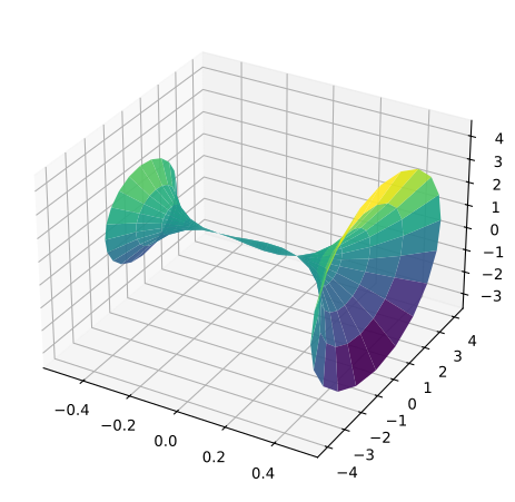
The Python that draws it

import json
import numpy as np
import matplotlib.pyplot as plt

# Surface recovered from the 2005 MATLAB figure "pahar".
# The mesh is 31x41, so the data ships alongside
# rather than being printed here.
data = json.load(open("pahar.json"))["series"][0]
X = np.array(data["x"]).reshape(data["x_shape"])
Y = np.array(data["y"]).reshape(data["y_shape"])
Z = np.array(data["z"], dtype=float)

fig = plt.figure(figsize=(6.4, 4.8))
ax = fig.add_subplot(111, projection="3d")
ax.plot_surface(X, Y, Z, cmap="viridis", linewidth=0)
ax.set_box_aspect((1, 1, 0.7))
fig.savefig("pahar.svg")    # SVG: sharp at any zoom

It reads its data from pahar.json — save that next to the script.

From the 2005 figure pahar.

Parallel lines

Lines of equal gradient never meet.

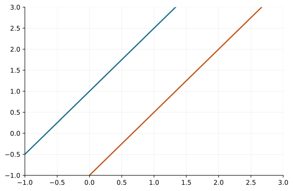
The Python that draws it

import numpy as np
import matplotlib.pyplot as plt

# 2 curve(s) recovered from the 2005 MATLAB figure "paralele"

x1 = np.array([
    -1, 0, 1, 2, 3, 4
])
y1 = np.array([
    -0.5, 1, 2.5, 4, 5.5, 7
])

x2 = np.array([
    -1, 0, 1, 2, 3, 4
])
y2 = np.array([
    -2.5, -1, 0.5, 2, 3.5, 5
])

fig, ax = plt.subplots(figsize=(6.4, 4.2))
ax.plot(x1, y1, lw=1.9)
ax.plot(x2, y2, lw=1.9)
ax.grid(True, lw=0.4, alpha=0.35)
ax.set_xlim(-1, 3)
ax.set_ylim(-1, 3)
ax.set_xlabel("x"); ax.set_ylabel("y")
fig.savefig("paralele.svg")    # SVG: sharp at any zoom

From the 2005 figure paralele.

Rotating y = cos x about an axis

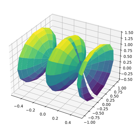
The Python that draws it

import json
import numpy as np
import matplotlib.pyplot as plt

# Surface recovered from the 2005 MATLAB figure "rot(cos)".
# The mesh is 64x41, so the data ships alongside
# rather than being printed here.
data = json.load(open("rot-cos-.json"))["series"][0]
X = np.array(data["x"]).reshape(data["x_shape"])
Y = np.array(data["y"]).reshape(data["y_shape"])
Z = np.array(data["z"], dtype=float)

fig = plt.figure(figsize=(6.4, 4.8))
ax = fig.add_subplot(111, projection="3d")
ax.plot_surface(X, Y, Z, cmap="viridis", linewidth=0)
ax.set_box_aspect((1, 1, 0.7))
fig.savefig("rot-cos-.svg")    # SVG: sharp at any zoom

It reads its data from rot-cos-.json — save that next to the script.

From the 2005 figure rot-cos-.

Rotating y = sin x about an axis

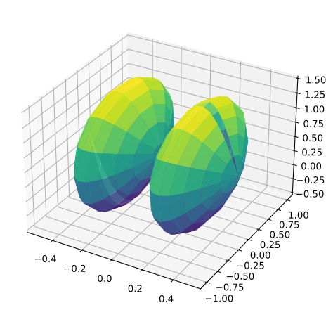
The Python that draws it

import json
import numpy as np
import matplotlib.pyplot as plt

# Surface recovered from the 2005 MATLAB figure "rot(sin)".
# The mesh is 64x41, so the data ships alongside
# rather than being printed here.
data = json.load(open("rot-sin-.json"))["series"][0]
X = np.array(data["x"]).reshape(data["x_shape"])
Y = np.array(data["y"]).reshape(data["y_shape"])
Z = np.array(data["z"], dtype=float)

fig = plt.figure(figsize=(6.4, 4.8))
ax = fig.add_subplot(111, projection="3d")
ax.plot_surface(X, Y, Z, cmap="viridis", linewidth=0)
ax.set_box_aspect((1, 1, 0.7))
fig.savefig("rot-sin-.svg")    # SVG: sharp at any zoom

It reads its data from rot-sin-.json — save that next to the script.

From the 2005 figure rot-sin-.

A truncated cone

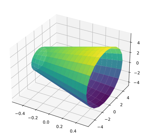
The Python that draws it

import json
import numpy as np
import matplotlib.pyplot as plt

# Surface recovered from the 2005 MATLAB figure "rot(trcon)".
# The mesh is 31x41, so the data ships alongside
# rather than being printed here.
data = json.load(open("rot-trcon-.json"))["series"][0]
X = np.array(data["x"]).reshape(data["x_shape"])
Y = np.array(data["y"]).reshape(data["y_shape"])
Z = np.array(data["z"], dtype=float)

fig = plt.figure(figsize=(6.4, 4.8))
ax = fig.add_subplot(111, projection="3d")
ax.plot_surface(X, Y, Z, cmap="viridis", linewidth=0)
ax.set_box_aspect((1, 1, 0.7))
fig.savefig("rot-trcon-.svg")    # SVG: sharp at any zoom

It reads its data from rot-trcon-.json — save that next to the script.

From the 2005 figure rot-trcon-.

Rotating y = x³ − x²

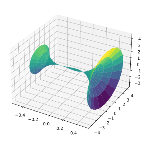
The Python that draws it

import json
import numpy as np
import matplotlib.pyplot as plt

# Surface recovered from the 2005 MATLAB figure "rot(x3-x2)".
# The mesh is 31x41, so the data ships alongside
# rather than being printed here.
data = json.load(open("rot-x3-x2-.json"))["series"][0]
X = np.array(data["x"]).reshape(data["x_shape"])
Y = np.array(data["y"]).reshape(data["y_shape"])
Z = np.array(data["z"], dtype=float)

fig = plt.figure(figsize=(6.4, 4.8))
ax = fig.add_subplot(111, projection="3d")
ax.plot_surface(X, Y, Z, cmap="viridis", linewidth=0)
ax.set_box_aspect((1, 1, 0.7))
fig.savefig("rot-x3-x2-.svg")    # SVG: sharp at any zoom

It reads its data from rot-x3-x2-.json — save that next to the script.

From the 2005 figure rot-x3-x2-.

Rotating y = x²

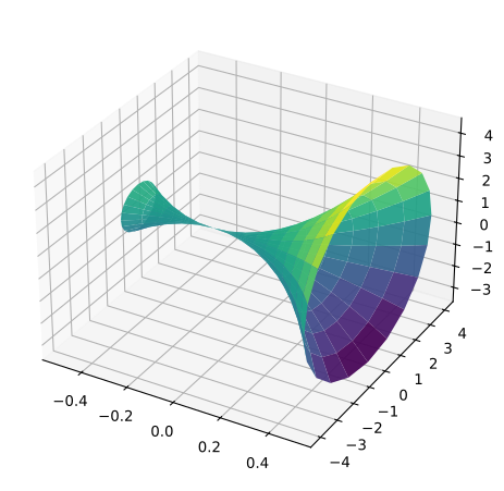
The Python that draws it

import json
import numpy as np
import matplotlib.pyplot as plt

# Surface recovered from the 2005 MATLAB figure "rot(xpatrat)".
# The mesh is 31x41, so the data ships alongside
# rather than being printed here.
data = json.load(open("rot-xpatrat-.json"))["series"][0]
X = np.array(data["x"]).reshape(data["x_shape"])
Y = np.array(data["y"]).reshape(data["y_shape"])
Z = np.array(data["z"], dtype=float)

fig = plt.figure(figsize=(6.4, 4.8))
ax = fig.add_subplot(111, projection="3d")
ax.plot_surface(X, Y, Z, cmap="viridis", linewidth=0)
ax.set_box_aspect((1, 1, 0.7))
fig.savefig("rot-xpatrat-.svg")    # SVG: sharp at any zoom

It reads its data from rot-xpatrat-.json — save that next to the script.

From the 2005 figure rot-xpatrat-.

Rotating y = x·sin x

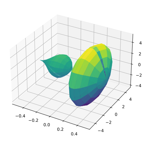
The Python that draws it

import json
import numpy as np
import matplotlib.pyplot as plt

# Surface recovered from the 2005 MATLAB figure "rot(xsinx)".
# The mesh is 64x41, so the data ships alongside
# rather than being printed here.
data = json.load(open("rot-xsinx-.json"))["series"][0]
X = np.array(data["x"]).reshape(data["x_shape"])
Y = np.array(data["y"]).reshape(data["y_shape"])
Z = np.array(data["z"], dtype=float)

fig = plt.figure(figsize=(6.4, 4.8))
ax = fig.add_subplot(111, projection="3d")
ax.plot_surface(X, Y, Z, cmap="viridis", linewidth=0)
ax.set_box_aspect((1, 1, 0.7))
fig.savefig("rot-xsinx-.svg")    # SVG: sharp at any zoom

It reads its data from rot-xsinx-.json — save that next to the script.

From the 2005 figure rot-xsinx-.

Solid of revolution

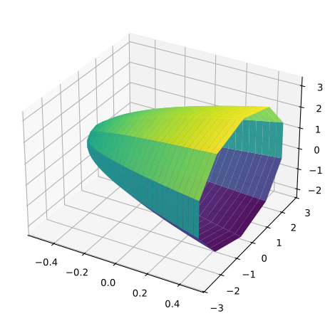
The Python that draws it

import json
import numpy as np
import matplotlib.pyplot as plt

# Surface recovered from the 2005 MATLAB figure "rot".
# The mesh is 81x31, so the data ships alongside
# rather than being printed here.
data = json.load(open("rot.json"))["series"][0]
X = np.array(data["x"]).reshape(data["x_shape"])
Y = np.array(data["y"]).reshape(data["y_shape"])
Z = np.array(data["z"], dtype=float)

fig = plt.figure(figsize=(6.4, 4.8))
ax = fig.add_subplot(111, projection="3d")
ax.plot_surface(X, Y, Z, cmap="viridis", linewidth=0)
ax.set_box_aspect((1, 1, 0.7))
fig.savefig("rot.svg")    # SVG: sharp at any zoom

It reads its data from rot.json — save that next to the script.

From the 2005 figure rot.

Solid of revolution

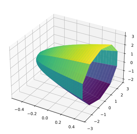
The Python that draws it

import json
import numpy as np
import matplotlib.pyplot as plt

# Surface recovered from the 2005 MATLAB figure "rot2".
# The mesh is 81x31, so the data ships alongside
# rather than being printed here.
data = json.load(open("rot2.json"))["series"][0]
X = np.array(data["x"]).reshape(data["x_shape"])
Y = np.array(data["y"]).reshape(data["y_shape"])
Z = np.array(data["z"], dtype=float)

fig = plt.figure(figsize=(6.4, 4.8))
ax = fig.add_subplot(111, projection="3d")
ax.plot_surface(X, Y, Z, cmap="viridis", linewidth=0)
ax.set_box_aspect((1, 1, 0.7))
fig.savefig("rot2.svg")    # SVG: sharp at any zoom

It reads its data from rot2.json — save that next to the script.

From the 2005 figure rot2.

Solid of revolution

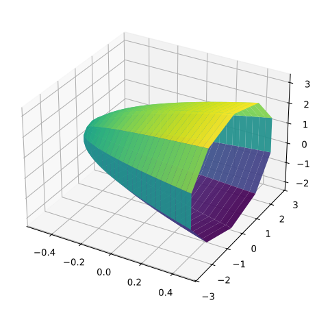
The Python that draws it

import json
import numpy as np
import matplotlib.pyplot as plt

# Surface recovered from the 2005 MATLAB figure "rot3".
# The mesh is 81x31, so the data ships alongside
# rather than being printed here.
data = json.load(open("rot3.json"))["series"][0]
X = np.array(data["x"]).reshape(data["x_shape"])
Y = np.array(data["y"]).reshape(data["y_shape"])
Z = np.array(data["z"], dtype=float)

fig = plt.figure(figsize=(6.4, 4.8))
ax = fig.add_subplot(111, projection="3d")
ax.plot_surface(X, Y, Z, cmap="viridis", linewidth=0)
ax.set_box_aspect((1, 1, 0.7))
fig.savefig("rot3.svg")    # SVG: sharp at any zoom

It reads its data from rot3.json — save that next to the script.

From the 2005 figure rot3.

Solid of revolution

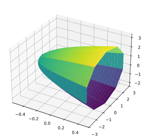
The Python that draws it

import json
import numpy as np
import matplotlib.pyplot as plt

# Surface recovered from the 2005 MATLAB figure "rot4(radical)".
# The mesh is 81x31, so the data ships alongside
# rather than being printed here.
data = json.load(open("rot4-radical-.json"))["series"][0]
X = np.array(data["x"]).reshape(data["x_shape"])
Y = np.array(data["y"]).reshape(data["y_shape"])
Z = np.array(data["z"], dtype=float)

fig = plt.figure(figsize=(6.4, 4.8))
ax = fig.add_subplot(111, projection="3d")
ax.plot_surface(X, Y, Z, cmap="viridis", linewidth=0)
ax.set_box_aspect((1, 1, 0.7))
fig.savefig("rot4-radical-.svg")    # SVG: sharp at any zoom

It reads its data from rot4-radical-.json — save that next to the script.

From the 2005 figure rot4-radical-.

Solid of revolution

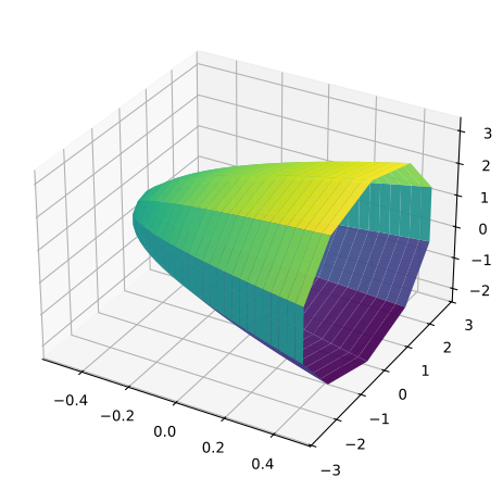
The Python that draws it

import json
import numpy as np
import matplotlib.pyplot as plt

# Surface recovered from the 2005 MATLAB figure "rot5(radical)".
# The mesh is 81x31, so the data ships alongside
# rather than being printed here.
data = json.load(open("rot5-radical-.json"))["series"][0]
X = np.array(data["x"]).reshape(data["x_shape"])
Y = np.array(data["y"]).reshape(data["y_shape"])
Z = np.array(data["z"], dtype=float)

fig = plt.figure(figsize=(6.4, 4.8))
ax = fig.add_subplot(111, projection="3d")
ax.plot_surface(X, Y, Z, cmap="viridis", linewidth=0)
ax.set_box_aspect((1, 1, 0.7))
fig.savefig("rot5-radical-.svg")    # SVG: sharp at any zoom

It reads its data from rot5-radical-.json — save that next to the script.

From the 2005 figure rot5-radical-.

Solid of revolution

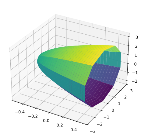
The Python that draws it

import json
import numpy as np
import matplotlib.pyplot as plt

# Surface recovered from the 2005 MATLAB figure "rot6(radical)".
# The mesh is 81x31, so the data ships alongside
# rather than being printed here.
data = json.load(open("rot6-radical-.json"))["series"][0]
X = np.array(data["x"]).reshape(data["x_shape"])
Y = np.array(data["y"]).reshape(data["y_shape"])
Z = np.array(data["z"], dtype=float)

fig = plt.figure(figsize=(6.4, 4.8))
ax = fig.add_subplot(111, projection="3d")
ax.plot_surface(X, Y, Z, cmap="viridis", linewidth=0)
ax.set_box_aspect((1, 1, 0.7))
fig.savefig("rot6-radical-.svg")    # SVG: sharp at any zoom

It reads its data from rot6-radical-.json — save that next to the script.

From the 2005 figure rot6-radical-.

Solid of revolution

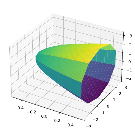
The Python that draws it

import json
import numpy as np
import matplotlib.pyplot as plt

# Surface recovered from the 2005 MATLAB figure "rot7(radical)".
# The mesh is 81x31, so the data ships alongside
# rather than being printed here.
data = json.load(open("rot7-radical-.json"))["series"][0]
X = np.array(data["x"]).reshape(data["x_shape"])
Y = np.array(data["y"]).reshape(data["y_shape"])
Z = np.array(data["z"], dtype=float)

fig = plt.figure(figsize=(6.4, 4.8))
ax = fig.add_subplot(111, projection="3d")
ax.plot_surface(X, Y, Z, cmap="viridis", linewidth=0)
ax.set_box_aspect((1, 1, 0.7))
fig.savefig("rot7-radical-.svg")    # SVG: sharp at any zoom

It reads its data from rot7-radical-.json — save that next to the script.

From the 2005 figure rot7-radical-.

Solid of revolution

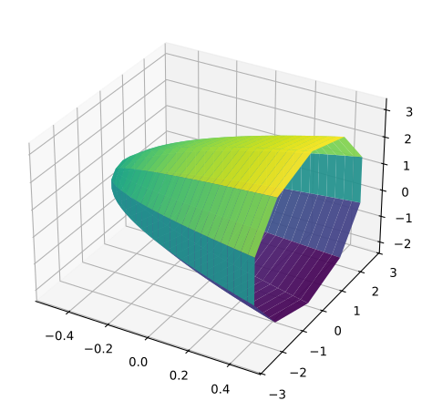
The Python that draws it

import json
import numpy as np
import matplotlib.pyplot as plt

# Surface recovered from the 2005 MATLAB figure "rot8(radical)".
# The mesh is 81x31, so the data ships alongside
# rather than being printed here.
data = json.load(open("rot8-radical-.json"))["series"][0]
X = np.array(data["x"]).reshape(data["x_shape"])
Y = np.array(data["y"]).reshape(data["y_shape"])
Z = np.array(data["z"], dtype=float)

fig = plt.figure(figsize=(6.4, 4.8))
ax = fig.add_subplot(111, projection="3d")
ax.plot_surface(X, Y, Z, cmap="viridis", linewidth=0)
ax.set_box_aspect((1, 1, 0.7))
fig.savefig("rot8-radical-.svg")    # SVG: sharp at any zoom

It reads its data from rot8-radical-.json — save that next to the script.

From the 2005 figure rot8-radical-.

Solid of revolution

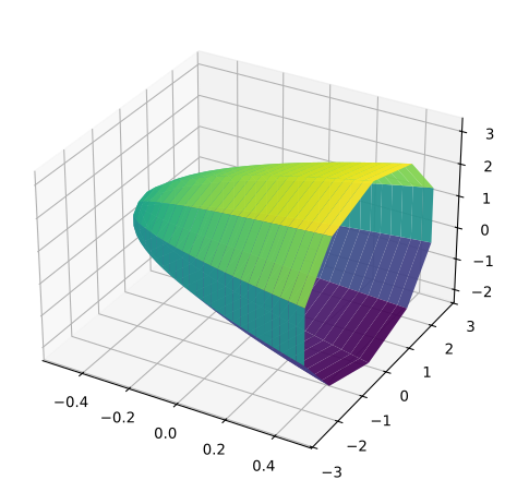
The Python that draws it

import json
import numpy as np
import matplotlib.pyplot as plt

# Surface recovered from the 2005 MATLAB figure "rot9(radical)".
# The mesh is 81x31, so the data ships alongside
# rather than being printed here.
data = json.load(open("rot9-radical-.json"))["series"][0]
X = np.array(data["x"]).reshape(data["x_shape"])
Y = np.array(data["y"]).reshape(data["y_shape"])
Z = np.array(data["z"], dtype=float)

fig = plt.figure(figsize=(6.4, 4.8))
ax = fig.add_subplot(111, projection="3d")
ax.plot_surface(X, Y, Z, cmap="viridis", linewidth=0)
ax.set_box_aspect((1, 1, 0.7))
fig.savefig("rot9-radical-.svg")    # SVG: sharp at any zoom

It reads its data from rot9-radical-.json — save that next to the script.

From the 2005 figure rot9-radical-.

y = x·sin x as a wireframe

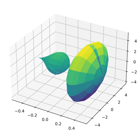
The Python that draws it

import json
import numpy as np
import matplotlib.pyplot as plt

# Surface recovered from the 2005 MATLAB figure "wire(xsinx)".
# The mesh is 64x41, so the data ships alongside
# rather than being printed here.
data = json.load(open("wire-xsinx-.json"))["series"][0]
X = np.array(data["x"]).reshape(data["x_shape"])
Y = np.array(data["y"]).reshape(data["y_shape"])
Z = np.array(data["z"], dtype=float)

fig = plt.figure(figsize=(6.4, 4.8))
ax = fig.add_subplot(111, projection="3d")
ax.plot_surface(X, Y, Z, cmap="viridis", linewidth=0)
ax.set_box_aspect((1, 1, 0.7))
fig.savefig("wire-xsinx-.svg")    # SVG: sharp at any zoom

It reads its data from wire-xsinx-.json — save that next to the script.

From the 2005 figure wire-xsinx-.

y = x³ − x²

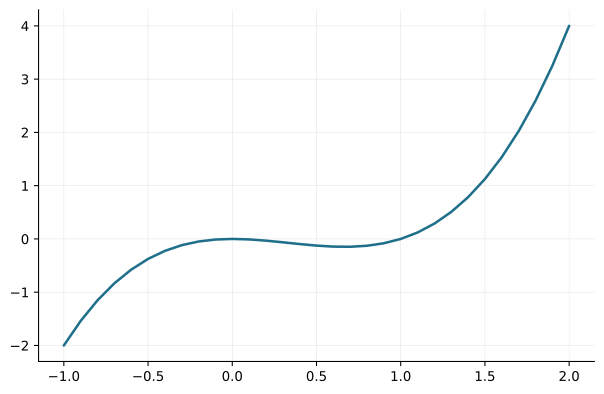
The Python that draws it

import numpy as np
import matplotlib.pyplot as plt

# 1 curve(s) recovered from the 2005 MATLAB figure "x3-x2"

x1 = np.array([
    -1, -0.9, -0.8, -0.7, -0.6, -0.5, -0.4, -0.3, -0.2, -0.1, 0, 0.1, 0.2,
    0.3, 0.4, 0.5, 0.6, 0.7, 0.8, 0.9, 1, 1.1, 1.2, 1.3, 1.4, 1.5, 1.6, 1.7,
    1.8, 1.9, 2
])
y1 = np.array([
    -2, -1.539, -1.152, -0.833, -0.576, -0.375, -0.224, -0.117, -0.048,
    -0.011, 0, -0.009, -0.032, -0.063, -0.096, -0.125, -0.144, -0.147,
    -0.128, -0.081, 0, 0.121, 0.288, 0.507, 0.784, 1.125, 1.536, 2.023,
    2.592, 3.249, 4
])

fig, ax = plt.subplots(figsize=(6.4, 4.2))
ax.plot(x1, y1, lw=1.9)
ax.grid(True, lw=0.4, alpha=0.35)
ax.set_xlabel("x"); ax.set_ylabel("y")
fig.savefig("x3-x2.svg")    # SVG: sharp at any zoom

From the 2005 figure x3-x2.