Complex numbers

The real numbers can solve first-degree equations $ax+b=0,$ $a,b\in \mathbb{R}\text{ cu }a\ne 0.$ They cannot, however, solve every second-degree equation with real coefficients; for example the equation ${{x}^{2}}+1=0.$ This calls for widening the notion of number so that, in the new set of numbers, every second-degree equation with real coefficients has solutions. That extension leads to the notion of a complex number.

A complex number has the form $z=a+ib,a,b\in R$, where ${{i}^{2}}=-1$; $\operatorname{Re}\left( z \right)=a$; $\operatorname{Im}\left( z \right)=b$.

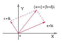
Representation of numbers in the complex plane:

$1+2i; 3+i; -2-3i; -2+i$

Plane vectors with their origin at the origin of the axes $(0,0)$ can be represented by a pair of real numbers $(a,b)$ (the tip of the vector). The complex number $z=a+ib$ is represented in the plane by the same point as the vector $(a,b)$.

Operations with complex numbers.

Let ${{z}_{1}}={{a}_{1}}+i{{b}_{1}}$ and ${{z}_{2}}={{a}_{2}}+i{{b}_{2}}$

${{z}_{1}}+{{z}_{2}}=\left( {{a}_{1}}+{{a}_{2}} \right)+i\left( {{b}_{1}}+{{b}_{2}} \right)$;

${{z}_{1}}{{z}_{2}}=\left( {{a}_{1}}{{a}_{2}}-{{b}_{1}}{{b}_{2}} \right)+i\left( {{a}_{1}}{{b}_{2}}+{{a}_{2}}{{b}_{1}} \right)$;

$\frac{1}{z}=\frac{a}{{{a}^{2}}+{{b}^{2}}}-i\frac{b}{{{a}^{2}}+{{b}^{2}}}$; $\frac{{{z}_{2}}}{{{z}_{1}}}=\frac{{{a}_{1}}{{a}_{2}}+{{b}_{1}}{{b}_{2}}}{a_{1}^{2}+b_{1}^{2}}-i\frac{{{a}_{1}}{{b}_{2}}-{{a}_{2}}{{b}_{1}}}{a_{1}^{2}+b_{1}^{2}}$;

Conjugate complex numbers

$\overline{z}=\overline{a+ib}=a-ib$ is called the conjugate of the complex number $z=a+ib$.

We have: a)$a=\frac{z+\overline{z}}{2}$; $ib=\frac{z-\overline{z}}{2}$; b)$z\in R$ if and only if $\overline{z}=z$;

c)$z$ is purely imaginary if and only if $\overline{z}=-z$; d)$\overline{\alpha z}=\alpha \cdot \overline{z},\forall \alpha \in R$

Let $z=a+ib$ and $z'=a'+ib'$ be two complex numbers. We have:

a)$\overline{z+z'}=\overline{z}+\overline{z'}$; b)$\overline{z\cdot z'}=\overline{z}\cdot \overline{z'}$; c)$\frac{z}{z'}=\frac{z\cdot \overline{z'}}{a{{'}^{2}}+b{{'}^{2}}}$,$z'\ne 0$.

The modulus of a complex number

Let $z\in C,z=a+ib,\left| z \right|=\rho =\sqrt{{{a}^{2}}+{{b}^{2}}}$

For every complex number $z\in C,z=a+ib$ we have:

1)$\left| z \right|\ge 0$; 2)$\left| z \right|=0\Leftrightarrow z=0$; 3)$z\cdot \overline{z}={{\left| z \right|}^{2}}$; 4)$\left| z \right|=\left| \overline{z} \right|$.

If ${{z}_{1}},{{z}_{2}}\in C$, then: 5)$\left| {{z}_{1}}\cdot {{z}_{2}} \right|=\left| {{z}_{1}} \right|\cdot \left| {{z}_{2}} \right|$; 6)$\left| \frac{{{z}_{1}}}{{{z}_{2}}} \right|=\left| \frac{{{z}_{1}}}{{{z}_{2}}} \right|,{{z}_{2}}\ne 0$;

7. The triangle inequality $\left| \left| {{z}_{1}} \right|-\left| {{z}_{2}} \right| \right|\le \left| {{z}_{1}}+{{z}_{2}} \right|\le \left| {{z}_{1}} \right|+\left| {{z}_{2}} \right|$.

Trigonometric form of a complex number

Let $z\in {{C}^{*}}$,$z=a+ib$. There exist unique $\rho =\left| z \right|=\sqrt{{{a}^{2}}+{{b}^{2}}}$ and $\phi \in \left[ 0,2\pi \right]$ such that: $z=\rho \left( \cos \phi +i\sin \phi \right)$; $\cos \phi =\frac{a}{\rho }$, $\sin \phi =\frac{b}{\rho }$.

Let ${{z}_{1}}={{\rho }_{1}}\left( \cos {{\phi }_{1}}+i\sin {{\phi }_{1}} \right)$ and ${{z}_{2}}={{\rho }_{2}}\left( \cos {{\phi }_{2}}+i\sin {{\phi }_{2}} \right)$

${{z}_{1}}{{z}_{2}}={{\rho }_{1}}{{\rho }_{2}}\left[ \cos \left( {{\phi }_{1}}+{{\phi }_{2}} \right)+i\sin \left( {{\phi }_{1}}+{{\phi }_{2}} \right) \right]$ $\frac{1}{{{z}_{1}}}=\frac{1}{{{\rho }_{1}}}\left[ \cos \left( -{{\phi }_{1}} \right)+i\sin \left( -{{\phi }_{1}} \right) \right]$

$\frac{{{z}_{2}}}{{{z}_{1}}}=\frac{{{\rho }_{2}}}{{{\rho }_{1}}}\left[ \cos \left( {{\varphi }_{2}}-{{\varphi }_{1}} \right)+i\sin \left( {{\varphi }_{2}}-{{\varphi }_{1}} \right) \right]$ $z_{1}^{n}=\rho _{1}^{n}\left( \cos n{{\varphi }_{1}}+i\sin n{{\varphi }_{1}} \right)$

$\sqrt[n]{{{z}_{1}}}=\sqrt[n]{{{\rho }_{1}}}\left( \cos \frac{{{\phi }_{1}}+2k\pi }{n}+i\sin \frac{{{\phi }_{1}}+2k\pi }{n} \right),n\in \left\{ 0,1,...,n-1 \right\}$

De Moivre's formula: ${{\left( \cos \varphi +i\sin \varphi \right)}^{n}}=\cos n\varphi +i\sin n\varphi ,n\in {{N}^{*}}$.

Expanding the left-hand side using the binomial theorem gives the following relation:

$\begin{aligned} & {{\cos }^{n}}\varphi +C_{n}^{2}{{\cos }^{n-2}}\varphi \cdot {{\sin }^{2}}\varphi +C_{n}^{4}{{\cos }^{n-4}}\varphi \cdot {{\sin }^{4}}\varphi +...+i(C_{n}^{1}{{\cos }^{n-1}}\varphi \cdot \sin \varphi +C_{n}^{3}{{\cos }^{n-3}}\varphi \cdot {{\sin }^{3}}\varphi +...)= \\ & =\cos n\varphi +i\sin n\varphi \\ \end{aligned}$ $\begin{aligned} & \cos n\varphi ={{\cos }^{n}}\varphi +C_{n}^{2}{{\cos }^{n-2}}\varphi \cdot {{\sin }^{2}}\varphi +C_{n}^{4}{{\cos }^{n-4}}\varphi \cdot {{\sin }^{4}}\varphi +...; \\ & \sin n\varphi =C_{n}^{1}{{\cos }^{n-1}}\varphi \cdot \sin \varphi +C_{n}^{3}{{\cos }^{n-3}}\varphi \cdot {{\sin }^{3}}\varphi +...; \\ & tgnu=\frac{C_{n}^{1}tg\varphi -C_{n}^{3}t{{g}^{3}}\varphi +C_{n}^{5}t{{g}^{5}}\varphi ...}{1-C_{n}^{2}t{{g}^{2}}\varphi +C_{n}^{4}t{{g}^{4}}\varphi -...} \\ \end{aligned}$

Euler's formula:

${{e}^{i\theta }}=\cos \theta +i\sin \theta$ so for $\theta =\pi \Rightarrow$ ${{e}^{i\cdot \pi }}=-1$ ${{e}^{-i\theta }}=\cos \theta -i\sin \theta$ ${{e}^{i\theta }}\cdot {{e}^{-i\theta }}=(\cos \theta +i\sin \theta )\cdot (\cos \theta -i\sin \theta )={{\cos }^{2}}\theta +{{\sin }^{2}}\theta =1$ $\left| {{e}^{i\theta }} \right|=1$.

Applications of complex numbers in geometry

The equation of the circle with centre ${{M}_{0}}\left( {{z}_{0}} \right)$ and radius $r>0$ is $\left| z-{{z}_{0}} \right|=r$

Let the points ${{M}_{1}}\left( {{z}_{1}} \right)$ and ${{M}_{2}}\left( {{z}_{2}} \right)$. We have $m\left( \sphericalangle {{M}_{2}}O{{M}_{1}} \right)=\arg \frac{{{z}_{2}}}{{{z}_{1}}}$.

Let the points ${{M}_{1}}\left( {{z}_{1}} \right)$, ${{M}_{2}}\left( {{z}_{2}} \right)$, ${{M}_{3}}\left( {{z}_{3}} \right)$. Then $m\left( \sphericalangle {{M}_{3}}{{M}_{1}}{{M}_{2}} \right)=\arg \frac{{{z}_{3}}-{{z}_{1}}}{{{z}_{2}}-{{z}_{1}}}$

Given the points ${{M}_{1}}\left( {{z}_{1}} \right)$, ${{M}_{2}}\left( {{z}_{2}} \right)$, ${{M}_{3}}\left( {{z}_{3}} \right)$, ${{M}_{4}}\left( {{z}_{4}} \right)$, the lines ${{M}_{1}}{{M}_{2}}$ and ${{M}_{3}}{{M}_{4}}$ are perpendicular if and only if $\frac{{{z}_{1}}-{{z}_{2}}}{{{z}_{3}}-{{z}_{4}}}$ is purely imaginary, that is $\operatorname{Re}\frac{{{z}_{1}}-{{z}_{2}}}{{{z}_{3}}-{{z}_{4}}}=0$.

The points ${{M}_{1}}\left( {{z}_{1}} \right)$, ${{M}_{2}}\left( {{z}_{2}} \right)$, ${{M}_{3}}\left( {{z}_{3}} \right)$, ${{M}_{4}}\left( {{z}_{4}} \right)$ are concyclic if and only if $\arg \frac{{{z}_{1}}-{{z}_{3}}}{{{z}_{2}}-{{z}_{3}}}-\arg \frac{{{z}_{1}}-{{z}_{4}}}{{{z}_{2}}-{{z}_{4}}}\in \left\{ 0,\pi \right\}$.

Two triangles ${{A}_{1}}{{A}_{2}}{{A}_{3}}$ and $A{{'}_{1}}A{{'}_{2}}A{{'}_{3}}$, with vertices of affix ${{z}_{k}}$ and $z{{'}_{k}},1\le k\le 3$ respectively, are similar if and only if: $\frac{{{z}_{2}}-{{z}_{1}}}{{{z}_{3}}-{{z}_{1}}}=\frac{z{{'}_{2}}-z{{'}_{1}}}{z{{'}_{3}}-z{{'}_{1}}}$.

The complex number $\varepsilon$

The cube roots of unity

The solutions of the equation ${{x}^{3}}-1=0$ are the complex roots of the polynomial $f={{x}^{3}}-1$, $f\in C\left[ x \right]$

${{x}^{3}}-1=(x-1)({{x}^{2}}+x+1)=0\Rightarrow$ $x-1=0;$

$\Rightarrow$ ${{x}_{1}}=1$

${{x}^{2}}+x+1=0$ $\Rightarrow$ $\Delta ={{b}^{2}}-4ac=1-4=-3\Rightarrow \Delta <0$

${{x}_{2,3}}=\frac{-b\pm i\sqrt{\left| \Delta \right|}}{2a}$ $\Rightarrow$ ${{x}_{2,3}}=\frac{-1\pm i\sqrt{3}}{2}$

We adopt the following notation:

$\varepsilon =-\frac{1}{2}+\frac{\sqrt{3}}{2}i={{x}_{2}}$ $\bar{\varepsilon }=-\frac{1}{2}-\frac{\sqrt{3}}{2}i={{x}_{3}}$

Properties:

${{\varepsilon }^{3}}=1$

${{\varepsilon }^{2}}+\varepsilon +1=0$

${{\varepsilon }^{2}}=-\varepsilon -1=\bar{\varepsilon }$

${{1}^{-1}}=1$, ${{\varepsilon }^{-1}}={{\varepsilon }^{2}}$, ${{({{\varepsilon }^{2}})}^{-1}}=\varepsilon$

$\begin{aligned} & {{\varepsilon }^{0}}=1 \\ & {{\varepsilon }^{1}}=\varepsilon \\ & {{\varepsilon }^{2}}={{\varepsilon }^{2}} \\ \end{aligned}$	$\begin{aligned} & {{\varepsilon }^{3}}=1 \\ & {{\varepsilon }^{4}}=\varepsilon \\ & {{\varepsilon }^{5}}={{\varepsilon }^{2}} \\ \end{aligned}$	$\begin{aligned} & {{\varepsilon }^{3k}}=1 \\ & {{\varepsilon }^{3k+1}}=\varepsilon \\ & {{\varepsilon }^{3k+2}}={{\varepsilon }^{2}} \\ \end{aligned}$

Trigonometric form of the complex number $\varepsilon$

${{x}^{3}}-1=0$ $\Rightarrow {{x}^{3}}=1\Rightarrow x=\sqrt[3]{1}$

$\sqrt[3]{1}=\cos (\frac{2k\pi }{3})+i\sin (\frac{2k\pi }{3}),$ $k=0,1,2$

for k=0 we have: $\sqrt[3]{1}=\cos (\frac{2k\pi }{3})+i\sin (\frac{2k\pi }{3})=\cos (\frac{2\cdot 0\cdot \pi }{3})+i\sin (\frac{2\cdot 0\cdot \pi }{3})=\cos (0)+i\sin (0)=1+i\cdot 0=1$ for k=1 we have: $\sqrt[3]{1}=\cos (\frac{2k\pi }{3})+i\sin (\frac{2k\pi }{3})=\cos (\frac{2\cdot 1\cdot \pi }{3})+i\sin (\frac{2\cdot 1\cdot \pi }{3})=\cos (\frac{2\pi }{3})+i\sin (\frac{2\pi }{3})=-\frac{1}{2}+i\frac{\sqrt{3}}{2}=\varepsilon$

for k=2 we have: $\sqrt[3]{1}=\cos (\frac{2k\pi }{3})+i\sin (\frac{2k\pi }{3})=\cos (\frac{2\cdot 2\cdot \pi }{3})+i\sin (\frac{2\cdot 2\cdot \pi }{3})=\cos (\frac{4\pi }{3})+i\sin (\frac{4\pi }{3})=-\frac{1}{2}-i\frac{\sqrt{3}}{2}=\bar{\varepsilon }$

Graphical representation of the cube roots:

Remark. The roots of the polynomial $f={{x}^{n}}-1$, $f\in C\left[ x \right]$, $n\in {{N}^{*}}$ are:

$\begin{aligned} & {{x}_{k}}=\cos (\frac{2k\pi }{n})+i\sin (\frac{2k\pi }{n}),k=0,1,2...n-1 \\ & {{x}_{0}}=1,{{x}_{1}}=\cos (\frac{2\pi }{n})+i\sin (\frac{2\pi }{n}),{{x}_{2}}=\cos (\frac{4\pi }{n})+i\sin (\frac{4\pi }{n}),...,{{x}_{n-1}}=\cos (\frac{2(n-1)\pi }{n})+i\sin (\frac{2(n-1)\pi }{n}). \\ \end{aligned}$

For n=6 we have the following roots:

$\begin{aligned} & {{x}_{0}}=1,\text{ }{{x}_{1}}=\cos \left( \frac{2\pi }{6} \right)+i\sin \left( \frac{2\pi }{6} \right),\text{ }{{x}_{2}}=\cos \left( \frac{4\pi }{6} \right)+i\sin \left( \frac{4\pi }{6} \right),\text{ }{{x}_{3}}=\cos \left( \frac{6\pi }{6} \right)+i\sin \left( \frac{6\pi }{6} \right), \\ & {{x}_{4}}=\cos \left( \frac{8\pi }{6} \right)+i\sin \left( \frac{8\pi }{6} \right),\text{ }{{x}_{5}}=\cos \left( \frac{10\pi }{6} \right)+i\sin \left( \frac{10\pi }{6} \right)\Rightarrow \\ \end{aligned}$

$\begin{aligned} & \Rightarrow {{x}_{0}}=1,\text{ }{{x}_{1}}=\cos \left( \frac{\pi }{3} \right)+i\sin \left( \frac{\pi }{3} \right),\text{ }{{x}_{2}}=\cos \left( \frac{2\pi }{3} \right)+i\sin \left( \frac{2\pi }{3} \right),\text{ }{{x}_{3}}=\cos \left( \pi \right)+i\sin \left( \pi \right), \\ & {{x}_{4}}=\cos \left( \frac{4\pi }{3} \right)+i\sin \left( \frac{4\pi }{3} \right),\text{ }{{x}_{5}}=\cos \left( \frac{5\pi }{3} \right)+i\sin \left( \frac{5\pi }{3} \right)\text{. } \\ \end{aligned}$

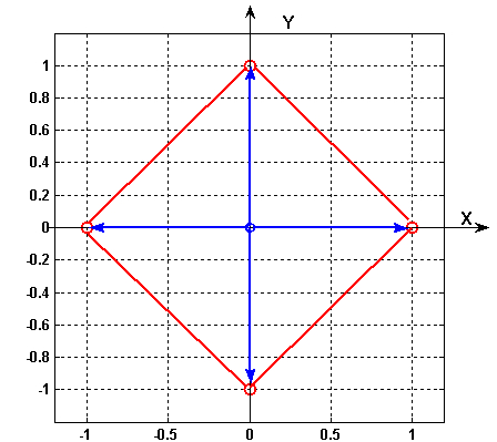
For n=4 we have the following roots:

$\begin{aligned} & {{x}_{0}}=1,\text{ }{{x}_{1}}=\cos \left( \frac{2\pi }{4} \right)+i\sin \left( \frac{2\pi }{4} \right), \\ & {{x}_{2}}=\cos \left( \frac{4\pi }{4} \right)+i\sin \left( \frac{4\pi }{4} \right),\text{ }{{x}_{3}}=\cos \left( \frac{6\pi }{4} \right)+i\sin \left( \frac{6\pi }{4} \right)\Rightarrow \\ & \Rightarrow {{x}_{0}}=1,\text{ }{{x}_{1}}=\cos \left( \frac{\pi }{2} \right)+i\sin \left( \frac{\pi }{2} \right), \\ & {{x}_{2}}=\cos \left( \pi \right)+i\sin \left( \pi \right),\text{ }{{x}_{3}}=\cos \left( \frac{3\pi }{2} \right)+i\sin \left( \frac{3\pi }{2} \right). \\ \end{aligned}$

${{\left( \sqrt[n]{-1} \right)}_{k}}=\cos \left( \frac{(2k+1)\pi }{n} \right)+i\sin \left( \frac{(2k+1)\pi }{n} \right),$ $k=0,1,2,...,n-1$

For brevity we use the following notation: ${{\left( \sqrt[n]{-1} \right)}_{k}}={{\omega }_{k}}$.

Graphical representation of the solutions of the equation ${{x}^{3}}+1=0$

${{x}^{3}}+1=0\Rightarrow {{x}^{3}}=-1\Rightarrow x=\sqrt[3]{-1}$

${{\omega }_{0}}=\cos \left( \frac{\pi }{3} \right)+i\sin \left( \frac{\pi }{3} \right)$

${{\omega }_{1}}=\cos \left( \frac{3\pi }{3} \right)+i\sin \left( \frac{3\pi }{3} \right)=\cos \left( \pi \right)+i\sin \left( \pi \right)=-1$

${{\omega }_{2}}=\cos \left( \frac{5\pi }{3} \right)+i\sin \left( \frac{5\pi }{3} \right)$