Powers and radicals

Year 9

Operations with real numbers

Natural powers of real numbers

1) ${{\left( +a \right)}^{n}}=+{{a}^{n}}$;

2) ${{\left( -a \right)}^{2n}}=+{{a}^{2n}}$;

3) ${{\left( -a \right)}^{2n+1}}=-{{a}^{2n+1}}$;

4) ${{a}^{m}}\cdot {{a}^{n}}={{a}^{m+n}}$;

5) ${{a}^{m}}:{{a}^{n}}={{a}^{m-n}},\,\,a\ne 0$;

6) ${{a}^{m}}\cdot {{b}^{m}}={{\left( a\cdot b \right)}^{m}}$;

7) ${{a}^{m}}:{{b}^{m}}={{\left( \frac{a}{b} \right)}^{m}},\,\,b\ne 0$;

8) $\frac{1}{{{a}^{m}}}={{\left( \frac{1}{a} \right)}^{m}}={{a}^{-m}},\,\,a\ne 0$;

9) ${{\left( {{a}^{m}} \right)}^{n}}={{a}^{m\cdot n}}={{\left( {{a}^{n}} \right)}^{m}}$;

10) ${{a}^{0}}=1,\,\,a\ne 0$;

11) ${{0}^{n}}=0,\,\,n\ne 0,\,\,n\in \Nu$.

Powers of real numbers extend to rational exponents, positive or negative, and to real exponents as well.

Fundamental identities

For any $x,y,z,t,a,b,c,d\in R$ and $n\in \Nu$, we have:

1) ${{a}^{2}}-{{b}^{2}}=\left( a-b \right)\left( a+b \right)\,;\,\,\text{ }4ab={{\left( a+b \right)}^{2}}-{{\left( a-b \right)}^{2}};$

2) ${{a}^{3}}-{{b}^{3}}=\left( a-b \right)\left( {{a}^{2}}+ab+{{b}^{2}} \right)\,;$

3) ${{a}^{3}}+{{b}^{3}}=\left( a+b \right)\left( {{a}^{2}}-ab+{{b}^{2}} \right)\,;$

4) ${{x}^{3}}+{{z}^{3}}+{{y}^{3}}-3xyz=\left( x+y+z \right)\left( {{x}^{2}}+{{y}^{2}}+{{z}^{2}}-xy-yz-zx \right)\,;$

5) ${{x}^{3}}+{{y}^{3}}+{{z}^{3}}={{\left( x+y+z \right)}^{3}}-3\left( x+y \right)\left( y+z \right)\left( z+x \right)\,;$

6) ${{a}^{5}}-{{b}^{5}}=\left( a-b \right)\left( {{a}^{4}}+{{a}^{3}}b+{{a}^{2}}{{b}^{2}}+a{{b}^{3}}+{{b}^{4}} \right)\,;$

7) ${{a}^{5}}+{{b}^{5}}=\left( a+b \right)\left( {{a}^{4}}-{{a}^{3}}b+{{a}^{2}}{{b}^{2}}-a{{b}^{3}}+{{b}^{4}} \right)\,;$

8) $\left( 1+a \right)\left( 1+{{a}^{2}}+{{a}^{4}} \right)=1+a+{{a}^{2}}+{{a}^{3}}+{{a}^{4}}+{{a}^{5}}\,;$

9) ${{a}^{n}}-{{b}^{n}}=\left( a-b \right)\left( {{a}^{n-1}}+{{a}^{n-2}}b+...+a{{b}^{n-2}}+{{b}^{n-1}} \right)\,;$

10) ${{a}^{2n}}-{{b}^{2n}}=\left( {{a}^{2}}-{{b}^{2}} \right)\left( {{a}^{2n-2}}+{{a}^{2n-4}}{{b}^{2}}+...+{{a}^{2}}{{b}^{2n-4}}+{{b}^{2n-2}} \right)\,;$

11) ${{a}^{2n+1}}+{{b}^{2n+1}}=\left( a+b \right)\left( {{a}^{2n}}+{{a}^{2n-1}}b+...+a{{b}^{2n-1}}+{{b}^{2n}} \right)\,;$

12) $\left( 1+a+{{a}^{2}}+...+{{a}^{n}} \right)\left( 1+{{a}^{n+1}} \right)=1+a+{{a}^{2}}+...+{{a}^{2n+1}}\,;$

Definition. Let A be a symmetric set and $f:A\to B$ a numerical function. The function f is called even if for $(\forall )x\in A$ we have $f(-x)=f(x)$. The function f is called odd if for $(\forall )x\in A$ we have $f(-x)=-f(x)$

Theorem. If n is even, the power function $f(x)={{x}^{n}}$ is an even function and its graph is symmetric about the OY axis. If n is odd, the power function $f(x)={{x}^{n}}$ is an odd function and its graph is symmetric about the origin.

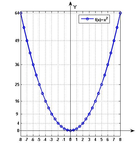
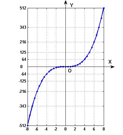
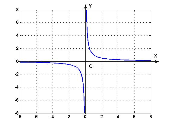
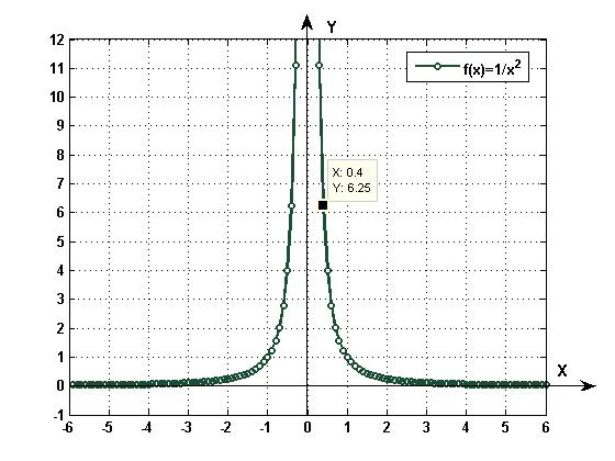
Graphs of the power functions $f(x)={{x}^{n}}$

1. if n=2 $\Rightarrow$ $f(x)={{x}^{2}}$ (parabola);

2. if n=3 $\Rightarrow$ $f(x)={{x}^{3}}$ (cubic parabola);

3. if n=-1 $\Rightarrow$ $f(x)={{x}^{-1}}=\frac{1}{x}$ (hyperbola);

4. if n=-1 $\Rightarrow$ $f(x)={{x}^{-2}}=\frac{1}{{{x}^{2}}}$ ;

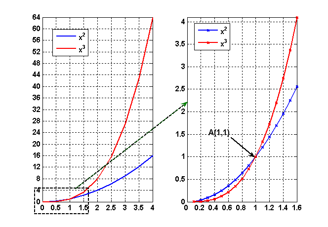
A comparison between the graphs of f(x)=x² and g(x)=x³: the left-hand graph shows the two functions on the interval [0,4], and the right-hand graph shows the same functions on the interval [0,1.6] after zooming in.

Radicals

Properties.

1.$\sqrt[m]{a}={{a}^{\frac{1}{m}}},\,\,\left( a>0 \right)$;

2.$\sqrt[m]{\frac{1}{a}}=\frac{1}{\sqrt[m]{a}}={{a}^{\frac{1}{m}}},\,\,\left( a>0 \right)$;

3.${{\left( \sqrt[m]{a} \right)}^{m}}=a,\,\,\left( a\ge 0 \right)$;

4.$\sqrt[m]{a}\cdot \sqrt[m]{b}=\sqrt[m]{ab},\,\,\left( a,b\ge 0 \right)$;

5.${{\left( \sqrt[m]{\frac{1}{a}} \right)}^{m}}=\frac{1}{a},\,\,\left( a>0 \right)$;

6.$\sqrt[m]{a}\cdot \sqrt[m]{b}\cdot \sqrt[m]{c}=\sqrt[m]{abc},\,\,\left( a,b,c\ge 0 \right)$;

7.$\sqrt[m]{a}:\sqrt[m]{b}=\sqrt[m]{\frac{a}{b}},\,\,\left( a\ge 0,b>0 \right)$;

8.$\sqrt[m]{a}\cdot \sqrt[n]{a}=\sqrt[mn]{{{a}^{m+n}}},\,\,\left( a\ge 0 \right)$;

9.$\sqrt[m]{a}:\sqrt[n]{a}=\sqrt[mn]{{{a}^{n-m}}},\,\,\left( a>0 \right)$;

10.$\sqrt[n]{{{a}^{nm}}}={{a}^{m}},\,\,\left( a\ge 0 \right)$;

11.$\sqrt[m]{{{a}^{n}}}={{\left( \sqrt[m]{a} \right)}^{n}}={{a}^{\frac{n}{m}}},\,\,\left( a\ge 0 \right)$;

12.$\sqrt[mn]{{{a}^{mp}}}=\sqrt[m]{{{a}^{p}}},\,\,\left( a>0 \right)$;

13.$\sqrt[m]{\sqrt[n]{a}}=\sqrt[mn]{a}=\sqrt[n]{\sqrt[m]{a}},\,\,\left( a\ge 0 \right)$;

14.$\sqrt[m]{{{a}^{p}}}:\sqrt[n]{{{b}^{q}}}=\sqrt[mn]{{{a}^{pn}}:{{b}^{qm}}},\,\,\left( a\ge 0,b>0 \right)$;

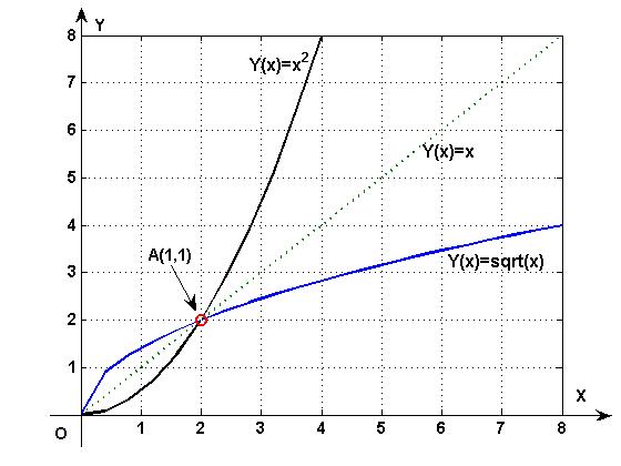
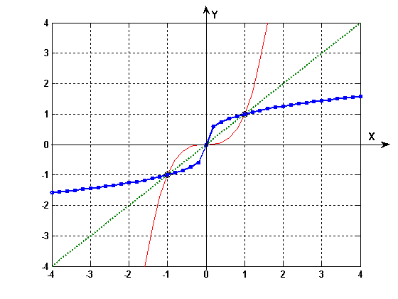
Graph of the radical function $y(x)=\sqrt[n]{x}$ and the graph of the inverse function ${{y}^{-1}}(x)={{x}^{n}}$

1. for n=2 $\Rightarrow y:[0,\infty )\to [0,\infty ),$ $y(x)=\sqrt{x,}$ ${{y}^{-1}}(x)={{x}^{2}}$; the function y(x) is strictly increasing and bijective on the interval $[0,\infty )$. The graph of the inverse function ${{y}^{-1}}(x)={{x}^{2}}$ is also shown. The two graphs are symmetric about the first bisector, the line $y(x)=x$, drawn dotted.

2. $y(x)={{x}^{3}}$ for n=3 $\Rightarrow y:\mathbb{R}\to \mathbb{R},$ $y(x)=\sqrt[3]{x}$ ${{y}^{-1}}(x)={{x}^{3}}$;

The modulus of a real number.

$\left| x \right|=\left\{ \begin{aligned} & x,\,\,dac\breve{a}\,\,x\ge 0 \\ & -x,\,\,dac\breve{a}\,\,x<0 \\ \end{aligned} \right.$

Properties: $\forall x,y\in R\,\,avem:$

1.$\left| x \right|=0\Leftrightarrow x=0$;

2.$\left| -x \right|=\left| x \right|$;

3.$\left| x \right|=\left| y \right|\Leftrightarrow x=y\,\,sau\,\,x=-y$;

4.; $\left| x \right|=a\Leftrightarrow x\in \{-a,\,a\},\,cu\,\,a\in R$

$\left| x \right|\le a\Leftrightarrow x\in [-a,\,a] ,\,cu\,\,a\in R$

$\left| x \right|\ge a\Leftrightarrow x\in [-\infty ,\,-a]\cup [a,\infty ] ,\,cu\,\,a\in R$

5.$-\left| x \right|\le x\le \left| x \right|$;

6.$\left| x+y \right|\le \left| x \right|+\left| y \right|$;

7.$\left| x-y \right|\le \left| x \right|-\left| y \right|$;

8.$\left| \left| x \right|-\left| y \right| \right|\le \left| x-y \right|$;

9.$\left| \left| x \right|-\left| y \right| \right|\le \left| x+y \right|\le \left| x \right|+\left| y \right|$;

10.$\left| xy \right|=\left| x \right|\cdot \left| y \right|$;

11.$\left| \frac{x}{y} \right|=\left| \frac{x}{y} \right|,\,\,\left( y\ne 0 \right)$;

12. $\sqrt{{{x}^{2}}}=\left| x \right|$

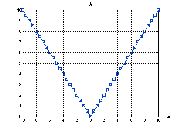
Graph of the function $f(x)=\left| x \right|$ , $(\forall )x\in \mathbb{R}$

Means

The arithmetic mean of the numbers a₁,a₂ . . a_n is $\frac{{{a}_{1}}+{{a}_{2}}+...+{{a}_{n}}}{n}$.

The harmonic mean of a₁,a₂ . . a_n is $\frac{\mathfrak{n}}{\frac{1}{{{a}_{1}}}+\frac{1}{a{}_{2}}+...+\frac{1}{{{a}_{n}}}}$, ${{a}_{n}}\in R_{+}^{*}$

The geometric mean of a₁,a₂ . . a_n is $\sqrt[n]{{{a}_{1}}{{a}_{2}}...{{a}_{n}}}$, ${{a}_{n}}\in R_{{}}^{*}$

The inequality of means. Let $n\in N,n\ge 2$ and ${{a}_{n}}\in R_{+}^{*}$; we have:

$\frac{\mathfrak{n}}{\frac{1}{{{a}_{1}}}+\frac{1}{a{}_{2}}+...+\frac{1}{{{a}_{n}}}}$ $\le$ $\sqrt[n]{{{a}_{1}}{{a}_{2}}...{{a}_{n}}}$ $\le$ $\frac{{{a}_{1}}+{{a}_{2}}+...+{{a}_{n}}}{n}$

The integer part of a number a is the largest integer smaller than the number a, written $[a]$. The fractional part of a number a is the difference between the number and its integer part, written $\{a\}$. We have $\{a\}=a-[a]$, $a=\{a\}+[a]$.

For $x\in \mathbb{R}$, we have $[x]\le x\le [x]+1;$ $x-1<[x]\le x;$

$0\le x<1;$

The signum (sign) function

$signum(x)=\operatorname{sgn} (x)=\left\{ \begin{aligned} & -1, x<0 \\ & 0, x=0 \\ & 1, x>0 \\ \end{aligned} \right.$